📖 Clustering Algorithms

🧭 Objective

• 🧠 What is Clustering?
• 📌 When is Clustering Useful?
• 📏 Evaluation Challenges

📦 Data Setup

• 📥 Load Dataset
• 🧹 Preprocessing

📊 Clustering Algorithms

📈 KMeans

🧱 Hierarchical Clustering

🌐 DBSCAN

🎲 Gaussian Mixture Models (GMM)

📍 Mean Shift

🎼 Spectral Clustering

📡 OPTICS

🌲 BIRCH

🔥 HDBSCAN

🧬 Affinity Propagation

📌 Summary Table

• 📋 Comparison Across Methods
• 🧭 Practical Recommendations

---

🧭 Objective

🧠 What is Clustering?

📖 Click to Expand

🧠 What is Clustering?

Clustering is an unsupervised learning technique that groups similar data points together without predefined labels.

• The goal is to identify natural groupings in data based on similarity or distance
• Each group is called a cluster, and the points within a cluster are more similar to each other than to points in other clusters
• Used to uncover structure in data when no labels are available

Types of Clustering

• Hard Clustering: Each point belongs to one cluster (e.g., KMeans)
• Soft Clustering: Points can belong to multiple clusters with probabilities (e.g., GMM)
• Hierarchical Clustering: Builds a tree-like structure of nested clusters
• Density-Based Clustering: Forms clusters based on dense regions (e.g., DBSCAN)

📌 When is Clustering Useful?

📖 Click to Expand

📌 When is Clustering Useful?

Clustering is helpful when you want to discover structure or patterns in unlabeled data.

Common Applications

• Customer Segmentation: Group users based on behavior or demographics
• Market Research: Identify distinct buyer personas
• Anomaly Detection: Spot outliers as points that don’t belong to any cluster
• Recommender Systems: Group similar items or users
• Document Clustering: Group similar news articles, reports, etc.
• Genetics & Bioinformatics: Group similar gene expressions or cell types

Key Benefit

Clustering helps reduce complexity by summarizing large datasets into meaningful groups, even when labels are unavailable.

📏 Evaluation Challenges

📖 Click to Expand

📏 Evaluation Challenges

Clustering is difficult to evaluate because it’s unsupervised — there’s no ground truth.

Internal Evaluation

• Silhouette Score: Measures how well a point fits within its cluster vs. others
• Davies-Bouldin Index: Lower values = better cluster separation
• Calinski-Harabasz Index: Ratio of between- to within-cluster dispersion

External Evaluation (when ground truth is available)

• Adjusted Rand Index (ARI): Measures similarity to true labels
• Normalized Mutual Information (NMI): Captures mutual information between assignments and labels

Other Challenges

• Choosing the Number of Clusters (K)
• Handling High-Dimensionality: PCA/t-SNE often needed
• Scale Sensitivity: Many algorithms need feature normalization
• Irregular Cluster Shapes: Some methods fail on non-spherical clusters

Back to the top

---

📦 Data Setup

📥 Load Dataset

from sklearn.datasets import make_blobs
import pandas as pd
import numpy as np
import matplotlib.pyplot as plt
import seaborn as sns

# Generate synthetic clusterable data
X, y = make_blobs(n_samples=500, centers=4, cluster_std=1.2, random_state=42)
df = pd.DataFrame(X, columns=["feature_1", "feature_2"])

# Plot raw input
plt.figure(figsize=(6, 4))
sns.scatterplot(data=df, x="feature_1", y="feature_2")
plt.title("Unlabeled Input Data")
plt.show()

🧹 Preprocessing

📖 Click to Expand

🧹 Preprocessing

Clustering algorithms like KMeans, DBSCAN, and GMM are sensitive to feature scale.

• We apply StandardScaler to normalize all features to zero mean and unit variance
• This ensures that distance-based calculations treat each feature equally
• Additional steps like missing value imputation or encoding are skipped here as all features are numeric and clean

from sklearn.preprocessing import StandardScaler

# Scale data
scaler = StandardScaler()
df_scaled = pd.DataFrame(scaler.fit_transform(df), columns=df.columns)

# Preview
df_scaled.head()

	feature_1	feature_2
0	-0.766161	0.562117
1	-1.266310	-1.545187
2	2.006315	-0.297524
3	0.077145	0.684294
4	-0.385682	-1.611826

Back to the top

---

📊 Clustering Algorithms

📊 Comparison

Algorithm	Works Well For	Assumes Shape	Needs Scaling	Handles Outliers	Notes
KMeans	Spherical, equal-size blobs	Spherical	✅ Yes	❌ No	Fast, interpretable
Hierarchical	Any size, low dims	Flexible (linkage)	🟡 Sometimes	❌ No	Good for visualizing nested groups
DBSCAN	Irregular, density-based	Arbitrary	✅ Yes	✅ Yes	Needs eps tuning
GMM	Elliptical, probabilistic	Gaussian blobs	✅ Yes	❌ No	Soft assignments
Mean Shift	Smooth cluster shapes	Arbitrary	✅ Yes	❌ No	Bandwidth sensitive
Spectral	Graph-connected data	Graph-based	✅ Yes	❌ No	Slow for large N
OPTICS	Nested, variable density	Arbitrary	🟡 Sometimes	✅ Yes	Better than DBSCAN for chaining
BIRCH	Large data, streaming	Spherical-ish	🟡 Sometimes	❌ No	Memory-efficient
HDBSCAN	Hierarchical + density	Arbitrary	🟡 Sometimes	✅ Yes	Adaptive to density
Affinity Prop.	Message-passing structure	N/A (similarity)	✅ Yes	❌ No	No need to set K

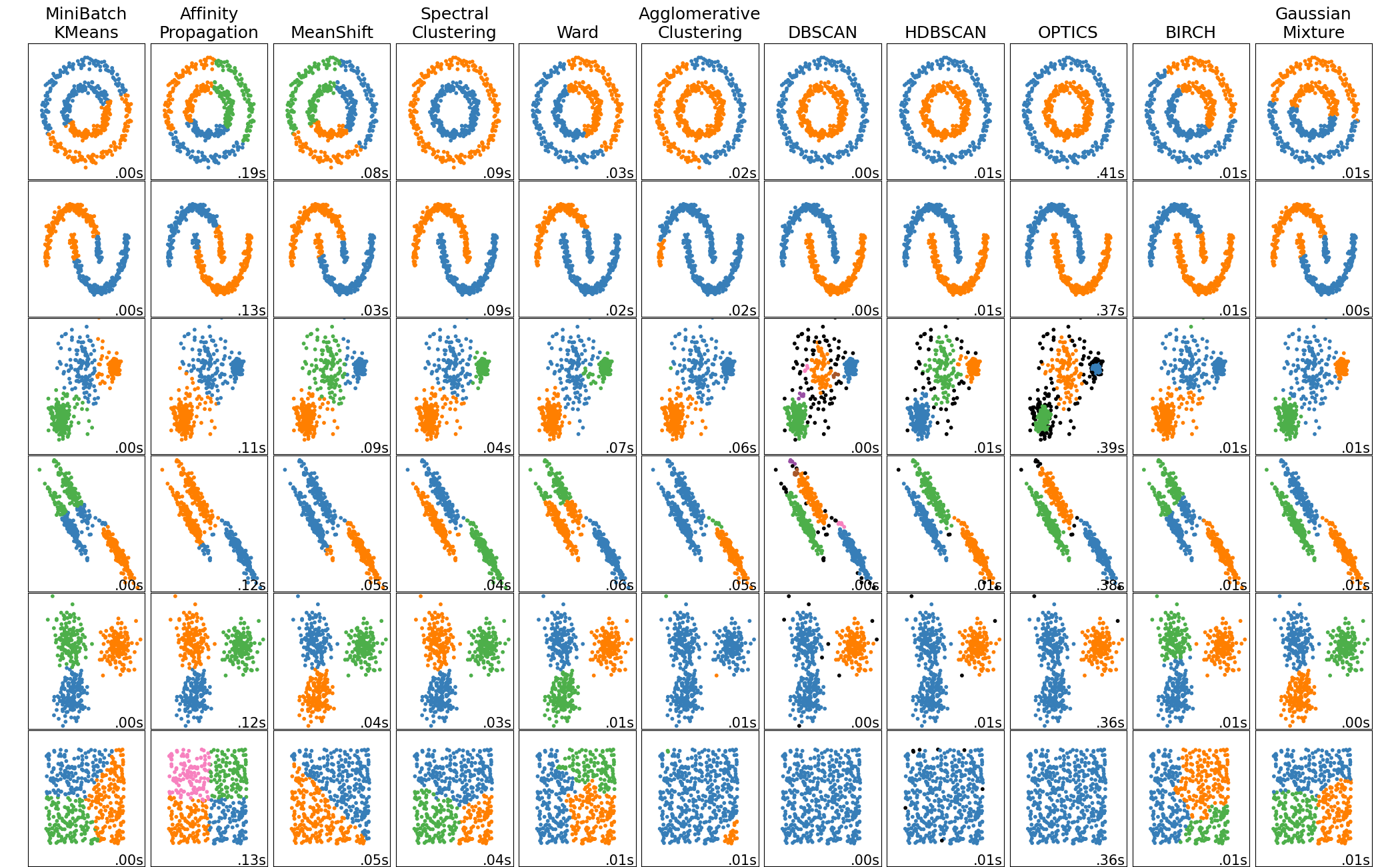
🖼️ Visual Comparison

This image from scikit-learn shows how different algorithms behave on varied shapes and densities:

Back to the top

---

📈 KMeans

📖 Click to Expand

📈 What is KMeans?

KMeans is a partitioning-based clustering algorithm that groups data into K clusters by minimizing the sum of squared distances (inertia) within clusters.

⚙️ How It Works

1. Initialize K centroids (randomly or via KMeans++)
2. Assign each point to the nearest centroid
3. Update centroids as the mean of all assigned points
4. Repeat steps 2–3 until convergence

✅ When to Use

• Clusters are compact, well-separated, and roughly spherical
• Scalability matters — KMeans is fast and efficient
• Applications like customer segmentation, image compression, etc.

⚠️ Limitations

• Requires choosing K in advance
• Sensitive to initial centroids, outliers, and feature scaling
• Assumes clusters are convex and isotropic

🧠 Variants

• KMeans++: Better centroid initialization
• MiniBatch KMeans: Faster for large datasets
• Fuzzy C-Means: Soft assignment to multiple clusters

⚙️ KMeans Config

# 📈 KMeans — ⚙️ Config
from sklearn.preprocessing import StandardScaler

# === CONFIG ===
k_range = range(2, 10)       # Range of K values to evaluate
k_final = 4                  # Final K to use when fitting the model
random_state = 42            # Seed for reproducibility
use_scaled_data = True       # Whether to scale before clustering
scaler = StandardScaler()    # Scaler object

# Prepare input data
df_input = df.copy()
if use_scaled_data:
    df_input = pd.DataFrame(scaler.fit_transform(df), columns=df.columns)

# Preview
df_input.head()

	feature_1	feature_2
0	-0.766161	0.562117
1	-1.266310	-1.545187
2	2.006315	-0.297524
3	0.077145	0.684294
4	-0.385682	-1.611826

📉 K Selection: Elbow + Silhouette

📖 Click to Expand

📉 K Selection Using Elbow + Silhouette

Choosing the right number of clusters (K) is critical to effective clustering.

🔹 Elbow Method

• Plots inertia (within-cluster sum of squares) vs. K
• Look for a point where the drop in inertia slows significantly — the "elbow"
• Simple and fast, but subjective

🔹 Silhouette Score

• Measures how well each point fits within its cluster vs. the next best
• Values range from -1 to 1:
  • Closer to 1 → well-clustered
  • Around 0 → overlapping clusters
  • Negative → likely misclassified
• Useful for identifying over-clustering or under-clustering

🔁 Best Practice

Use both methods together:

• Elbow narrows the K range
• Silhouette refines the choice based on structure quality

from sklearn.cluster import KMeans
from sklearn.metrics import silhouette_score
import matplotlib.pyplot as plt

inertias = []
silhouettes = []

for k in k_range:
    kmeans = KMeans(n_clusters=k, n_init=10, random_state=random_state)
    labels = kmeans.fit_predict(df_input)
    inertias.append(kmeans.inertia_)
    silhouettes.append(silhouette_score(df_input, labels))

# Plot Elbow and Silhouette Score
fig, ax = plt.subplots(1, 2, figsize=(12, 4))

# Elbow plot
ax[0].plot(list(k_range), inertias, marker='o')
ax[0].set_title("Elbow Method (Inertia vs K)")
ax[0].set_xlabel("Number of Clusters (K)")
ax[0].set_ylabel("Inertia")

# Silhouette plot
ax[1].plot(list(k_range), silhouettes, marker='o', color='green')
ax[1].set_title("Silhouette Score vs K")
ax[1].set_xlabel("Number of Clusters (K)")
ax[1].set_ylabel("Silhouette Score")

plt.tight_layout()
plt.show()

🚀 Run KMeans

# Fit KMeans using the selected final K
kmeans_final = KMeans(n_clusters=k_final, n_init=10, random_state=random_state)
labels_final = kmeans_final.fit_predict(df_input)

# Append cluster assignments to the data
df_kmeans = df_input.copy()
df_kmeans["cluster"] = labels_final
df_kmeans.head()

	feature_1	feature_2	cluster
0	-0.766161	0.562117	1
1	-1.266310	-1.545187	2
2	2.006315	-0.297524	0
3	0.077145	0.684294	3
4	-0.385682	-1.611826	2

# Show cluster counts
print(df_kmeans["cluster"].value_counts().sort_index())

0    125
1    125
2    125
3    125
Name: cluster, dtype: int64

📊 Visualize Clusters

def plot_clusters_2d(df, label_col="cluster", centroids=None, title="Cluster Visualization (2D)", hue_palette="tab10"):
    """
    Plots a 2D scatterplot of clusters with optional centroids.

    Parameters:
        df (pd.DataFrame): DataFrame with exactly 2 feature columns and a cluster label column.
        label_col (str): Name of the column containing cluster labels.
        centroids (ndarray or list): Optional array of centroid coordinates (shape: [K, 2]).
        title (str): Plot title.
        hue_palette (str): Color palette for clusters.
    """
    plt.figure(figsize=(6, 5))
    sns.scatterplot(data=df, x=df.columns[0], y=df.columns[1], hue=label_col, palette=hue_palette, s=50, edgecolor="k")

    if centroids is not None:
        plt.scatter(centroids[:, 0], centroids[:, 1], c='black', s=150, marker='X', label='Centroids')

    plt.title(title)
    plt.legend()
    plt.show()

plot_clusters_2d(df_kmeans, label_col="cluster", centroids=kmeans_final.cluster_centers_, title=f"KMeans Clustering (K = {k_final})")

from sklearn.decomposition import PCA
import matplotlib.pyplot as plt
import seaborn as sns

def plot_clusters_pca(df_with_labels, label_col="cluster", title="Cluster Visualization (PCA-backed)"):
    """
    Plots clusters in 2D using PCA if necessary.

    Parameters:
        df_with_labels (pd.DataFrame): DataFrame with features + cluster label column.
        label_col (str): Name of the cluster label column.
        title (str): Plot title.
    """
    features = df_with_labels.drop(columns=[label_col])

    # Reduce to 2D if needed
    if features.shape[1] > 2:
        pca = PCA(n_components=2, random_state=42)
        reduced = pca.fit_transform(features)
        plot_df = pd.DataFrame(reduced, columns=["PC1", "PC2"])
    else:
        plot_df = features.copy()
        plot_df.columns = ["PC1", "PC2"]

    plot_df[label_col] = df_with_labels[label_col].values

    plt.figure(figsize=(6, 5))
    sns.scatterplot(data=plot_df, x="PC1", y="PC2", hue=label_col, palette="tab10", s=50, edgecolor="k")
    plt.title(title)
    plt.show()
plot_clusters_pca(df_kmeans, label_col="cluster", title=f"KMeans Clustering (K = {k_final})")

📌 Cluster Summary

import pandas as pd
import matplotlib.pyplot as plt
import seaborn as sns

def summarize_clusters(df, label_col="cluster", summary_cols=None, cmap="Blues"):
    """
    Displays summary statistics for each cluster.

    Parameters:
        df (pd.DataFrame): DataFrame with features + cluster label.
        label_col (str): Column name containing cluster labels.
        summary_cols (list): List of columns to summarize. If None, all numeric features are used.
        cmap (str): Color map for background gradient.
    """
    if summary_cols is None:
        summary_cols = [col for col in df.select_dtypes(include="number").columns if col != label_col]

    summary = df.groupby(label_col).agg(
        count=(label_col, "size"),
        **{f"avg_{col}": (col, "mean") for col in summary_cols}
    ).reset_index()

    return summary.style.background_gradient(cmap=cmap, axis=0)
summarize_clusters(df_kmeans)

	cluster	count	avg_feature_1	avg_feature_2
0	0	125	1.530125	-0.154559
1	1	125	-0.990375	0.719419
2	2	125	-0.684463	-1.539546
3	3	125	0.144713	0.974686

Back to the top

---

🧱 Hierarchical Clustering

📖 Click to Expand

🧱 What is Hierarchical Clustering?

Hierarchical clustering builds a nested tree of clusters by either:

• Agglomerative (bottom-up): Merge closest clusters until one remains
• Divisive (top-down): Start with one big cluster and recursively split

It does not require you to predefine the number of clusters — instead, you choose where to “cut” the tree.

🔹 Distance Between Clusters (Linkage Types)

• Single linkage: Minimum distance between points in two clusters
• Complete linkage: Maximum distance
• Average linkage: Mean pairwise distance
• Ward linkage: Minimizes increase in total variance (best for compact clusters)

✅ When to Use

• You want a visual tree of how data groups form
• You’re unsure how many clusters to choose — let the tree reveal it
• You want interpretable cluster evolution (e.g., customer groups merging)

⚠️ Limitations

• Memory and time intensive for large datasets
• Sensitive to scale and noise
• Tree depth can be misleading without proper distance normalization

⚙️ Hierarchical Config

from sklearn.preprocessing import StandardScaler

# === CONFIG ===
hierarchical_metric = "euclidean"      # Distance metric (euclidean, manhattan, etc.)
hierarchical_linkage = "ward"          # Linkage: ward, single, complete, average
n_clusters_hierarchical = 4            # Number of clusters to cut the tree at
use_scaled_data_hierarchical = True    # Whether to scale features

# Prepare data
df_input_hier = df.copy()
if use_scaled_data_hierarchical:
    scaler_hier = StandardScaler()
    df_input_hier = pd.DataFrame(scaler_hier.fit_transform(df), columns=df.columns)

df_input_hier.head()

	feature_1	feature_2
0	-0.766161	0.562117
1	-1.266310	-1.545187
2	2.006315	-0.297524
3	0.077145	0.684294
4	-0.385682	-1.611826

🌳 Plot Dendrogram

📖 Click to Expand

🌳 What is a Dendrogram?

A dendrogram is a tree diagram that shows how points are merged into clusters during agglomerative clustering.

• X-axis: data points or their indexes
• Y-axis: distance between merged clusters
• You can “cut” the tree at any height to form flat clusters

🔍 Why It’s Useful

• Visualizes the entire clustering process, not just final clusters
• Helps choose the optimal number of clusters based on vertical gaps
• Useful when you don’t know how many clusters to use up front

from scipy.cluster.hierarchy import dendrogram, linkage
import matplotlib.pyplot as plt

# Compute linkage matrix
linkage_matrix = linkage(df_input_hier, method=hierarchical_linkage, metric=hierarchical_metric)

# Plot dendrogram
plt.figure(figsize=(10, 4))
dendrogram(linkage_matrix, truncate_mode='level', p=10)
plt.title(f"Hierarchical Dendrogram ({hierarchical_linkage.title()} Linkage)")
plt.xlabel("Data Points")
plt.ylabel(f"{hierarchical_metric.title()} Distance")
plt.show()

✂️ Choose Clusters from Tree

📖 Click to Expand

✂️ Cutting the Dendrogram into Flat Clusters

Once the hierarchical tree (dendrogram) is built, we flatten it into K clusters using a cutting rule.

🔧 How It Works

• The dendrogram represents how clusters were merged based on distance
• We choose a number K, and cut the tree horizontally to extract K flat clusters
• Internally, this is done using:
  • criterion='maxclust': Find the highest level where K clusters exist
  • t=K: The number of clusters to form

🧠 Key Benefit

• Lets you defer the choice of K until after seeing the full tree
• Supports exploratory workflows (e.g., try K = 3, 4, 5 and compare)

⚠️ Notes

• If clusters are very unbalanced or chaining happens, some clusters may be very small
• A good “cut height” usually corresponds to large vertical gaps in the dendrogram

# Recompute linkage_matrix if not already defined
from scipy.cluster.hierarchy import linkage, fcluster

linkage_matrix = linkage(df_input_hier, method=hierarchical_linkage, metric=hierarchical_metric)

# Cut the tree
labels_hier = fcluster(linkage_matrix, t=n_clusters_hierarchical, criterion='maxclust')

# Add to dataframe
df_hier = df_input_hier.copy()
df_hier["cluster"] = labels_hier

# Cluster counts
df_hier["cluster"].value_counts().sort_index()

1    125
2    125
3    126
4    124
Name: cluster, dtype: int64

📊 Visualize Clusters (PCA-backed)

plot_clusters_pca(df_hier, label_col="cluster", title="Hierarchical Clustering (PCA-backed)")
plot_clusters_2d(df_hier, label_col="cluster", title="Hierarchical Clustering (2D)")

📌 Cluster Summary

summarize_clusters(df_hier)

	cluster	count	avg_feature_1	avg_feature_2
0	1	125	-0.684463	-1.539546
1	2	125	1.530125	-0.154559
2	3	126	-0.985897	0.722557
3	4	124	0.149316	0.973557

Back to the top

---

🌐 DBSCAN

🌐 DBSCAN

📖 Click to Expand

🌐 What is DBSCAN?

DBSCAN (Density-Based Spatial Clustering of Applications with Noise) groups points into clusters based on density.

• Points in high-density areas → core points
• Border points are near core points
• Noise points are too isolated to join any cluster

🔧 Key Parameters

• eps: Radius for neighborhood search
• min_samples: Minimum neighbors to form a dense region

✅ When to Use

• You expect irregularly shaped clusters
• You want to automatically detect outliers
• No need to specify K upfront

⚠️ Limitations

• Requires careful tuning of eps
• Sensitive to feature scaling
• Struggles when density varies too much across regions

⚙️ DBSCAN Config

from sklearn.preprocessing import StandardScaler

# === CONFIG ===
dbscan_eps = 0.5                # Radius for neighbors
dbscan_min_samples = 5          # Minimum points to form a dense region
use_scaled_data_dbscan = True

# Prepare input
df_input_dbscan = df.copy()
if use_scaled_data_dbscan:
    scaler_db = StandardScaler()
    df_input_dbscan = pd.DataFrame(scaler_db.fit_transform(df), columns=df.columns)

🚀 Run DBSCAN

from sklearn.cluster import DBSCAN

# Fit DBSCAN
dbscan = DBSCAN(eps=dbscan_eps, min_samples=dbscan_min_samples)
labels_dbscan = dbscan.fit_predict(df_input_dbscan)

# Assign labels
df_dbscan = df_input_dbscan.copy()
df_dbscan["cluster"] = labels_dbscan
df_dbscan

	feature_1	feature_2	cluster
0	-0.766161	0.562117	0
1	-1.266310	-1.545187	1
2	2.006315	-0.297524	2
3	0.077145	0.684294	0
4	-0.385682	-1.611826	1
...	...	...	...
495	-0.709665	0.868735	0
496	0.148308	1.024226	0
497	-0.732909	-1.220579	1
498	-0.775140	-1.337366	1
499	1.628939	0.143440	2

500 rows × 3 columns

📊 Visual Output

plot_clusters_2d(df_dbscan, label_col="cluster", title="DBSCAN Clustering (2D)")

plot_clusters_pca(df_dbscan, label_col="cluster", title="DBSCAN Clustering (PCA-backed)")

📌 Cluster Summary

summarize_clusters(df_dbscan)

	cluster	count	avg_feature_1	avg_feature_2
0	0	250	-0.422831	0.847053
1	1	125	-0.684463	-1.539546
2	2	125	1.530125	-0.154559

Back to the top

---

🎲 Gaussian Mixture Models (GMM)

🎲 Gaussian Mixture Models (GMM)

📖 Click to Expand

🎲 What is GMM?

GMM is a probabilistic clustering method that assumes data is generated from a mixture of several Gaussian distributions.

• Each cluster is a Gaussian component defined by its own mean and covariance
• Unlike KMeans, it produces soft assignments (probabilities)

✅ When to Use

• Clusters may overlap and have elliptical shapes
• You need probabilistic membership, not just hard labels
• Ideal for continuous numeric features

⚙️ Key Parameters

• n_components: Number of clusters
• covariance_type: Full, tied, diagonal, spherical
• random_state: For reproducibility

⚠️ Limitations

• Assumes Gaussian-shaped clusters
• Sensitive to initial guesses and scaling
• Can overfit if too many components

⚙️ GMM Config

# === CONFIG ===
gmm_components = 4
gmm_covariance_type = "full"
use_scaled_data_gmm = True

# Prepare input
df_input_gmm = df.copy()
if use_scaled_data_gmm:
    scaler_gmm = StandardScaler()
    df_input_gmm = pd.DataFrame(scaler_gmm.fit_transform(df), columns=df.columns)

🚀 Run GMM

from sklearn.mixture import GaussianMixture

# Fit GMM
gmm = GaussianMixture(n_components=gmm_components, covariance_type=gmm_covariance_type, random_state=42)
labels_gmm = gmm.fit_predict(df_input_gmm)

# Assign labels
df_gmm = df_input_gmm.copy()
df_gmm["cluster"] = labels_gmm

📊 Visualize Clusters (PCA-backed)

plot_clusters_pca(df_gmm, label_col="cluster", title="GMM Clustering (PCA-backed)")
plot_clusters_2d(df_gmm, label_col="cluster", title="GMM Clustering (2D)")

📌 Cluster Summary

summarize_clusters(df_gmm)

	cluster	count	avg_feature_1	avg_feature_2
0	0	125	1.530125	-0.154559
1	1	125	-0.990375	0.719419
2	2	125	-0.684463	-1.539546
3	3	125	0.144713	0.974686

Back to the top

---

📍 Mean Shift

📍 Mean Shift

📖 Click to Expand

📍 What is Mean Shift?

Mean Shift is a centroid-based clustering algorithm that locates high-density regions (modes) by shifting points toward the mean of their local neighborhood.

• No need to specify number of clusters (K)
• Each data point moves to the densest area until convergence

✅ When to Use

• You want automatic cluster count detection
• Data has dense blobs or modes
• Good for small-to-medium datasets

⚙️ Key Parameters

• bandwidth: Radius of the neighborhood (if not provided, it's estimated)
• bin_seeding: Speed optimization using binning

⚠️ Limitations

• Computationally expensive
• Highly sensitive to bandwidth
• Doesn’t scale well for high dimensions

⚙️ Mean Shift Config

use_scaled_data_meanshift = True

# Prepare input
df_input_meanshift = df.copy()
if use_scaled_data_meanshift:
    scaler_ms = StandardScaler()
    df_input_meanshift = pd.DataFrame(scaler_ms.fit_transform(df), columns=df.columns)

🚀 Run Mean Shift

from sklearn.cluster import MeanShift, estimate_bandwidth

# Estimate bandwidth
bandwidth = estimate_bandwidth(df_input_meanshift, quantile=0.2, n_samples=200)

# Fit MeanShift
meanshift = MeanShift(bandwidth=bandwidth, bin_seeding=True)
labels_meanshift = meanshift.fit_predict(df_input_meanshift)

# Assign labels
df_meanshift = df_input_meanshift.copy()
df_meanshift["cluster"] = labels_meanshift

📊 Visualize Clusters (PCA-backed)

plot_clusters_pca(df_meanshift, label_col="cluster", title="Mean Shift Clustering (PCA-backed)")
# or if 2D:
plot_clusters_2d(df_meanshift, label_col="cluster", title="Mean Shift Clustering (2D)")

📌 Cluster Summary

summarize_clusters(df_meanshift)

	cluster	count	avg_feature_1	avg_feature_2
0	0	125	-0.990375	0.719419
1	1	125	1.530125	-0.154559
2	2	125	0.144713	0.974686
3	3	125	-0.684463	-1.539546

Back to the top

---

🎼 Spectral Clustering

📖 Click to Expand

🎼 What is Spectral Clustering?

Spectral clustering transforms the data into a graph of similarities, then finds clusters by analyzing the eigenvectors of the graph Laplacian.

• Works well for non-convex and irregular cluster shapes
• Doesn’t assume globular structure like KMeans

✅ When to Use

• When data has nonlinear structure (e.g., concentric circles)
• For small-to-medium datasets
• When traditional clustering fails on irregular shapes

⚙️ Key Parameters

• n_clusters: Number of output clusters
• affinity: Similarity measure (e.g., 'rbf', 'nearest_neighbors')
• assign_labels: Method to assign final clusters ('kmeans', 'discretize')

⚠️ Limitations

• Slow for large datasets (due to eigen decomposition)
• Needs tuning of affinity or neighbors
• Doesn't scale well beyond a few thousand points

⚙️ Spectral Config

spectral_clusters = 4
spectral_affinity = "rbf"         # or 'nearest_neighbors'
use_scaled_data_spectral = True

# Prepare input
df_input_spectral = df.copy()
if use_scaled_data_spectral:
    scaler_spectral = StandardScaler()
    df_input_spectral = pd.DataFrame(scaler_spectral.fit_transform(df), columns=df.columns)

🚀 Run Spectral Clustering

from sklearn.cluster import SpectralClustering

# Fit model
spectral = SpectralClustering(n_clusters=spectral_clusters,
                               affinity=spectral_affinity,
                               assign_labels="kmeans",
                               random_state=42)
labels_spectral = spectral.fit_predict(df_input_spectral)

# Assign labels
df_spectral = df_input_spectral.copy()
df_spectral["cluster"] = labels_spectral

📊 Visualize Clusters (PCA-backed)

plot_clusters_pca(df_spectral, label_col="cluster", title="Spectral Clustering (PCA-backed)")
# or if 2D:
plot_clusters_2d(df_spectral, label_col="cluster", title="Spectral Clustering (2D)")

📌 Cluster Summary

summarize_clusters(df_spectral)

	cluster	count	avg_feature_1	avg_feature_2
0	0	125	-0.684463	-1.539546
1	1	125	0.144713	0.974686
2	2	125	1.530125	-0.154559
3	3	125	-0.990375	0.719419

Back to the top

---

📡 OPTICS

📡 OPTICS

📖 Click to Expand

📡 What is OPTICS?

OPTICS (Ordering Points To Identify the Clustering Structure) is a density-based clustering algorithm similar to DBSCAN but more robust.

• Unlike DBSCAN, OPTICS doesn’t force you to set a fixed eps radius
• It builds a reachability plot to identify clusters of varying density

✅ When to Use

• When DBSCAN fails due to mixed-density clusters
• You want to extract nested or chained cluster structures

⚙️ Key Parameters

• min_samples: Minimum points in a neighborhood to form a core point
• xi: Sensitivity for extracting flat clusters from reachability structure

⚠️ Limitations

• Slower than DBSCAN for large datasets
• Still needs thoughtful tuning of min_samples and xi

⚙️ OPTICS Config

optics_min_samples = 5
optics_xi = 0.05
use_scaled_data_optics = True

df_input_optics = df.copy()
if use_scaled_data_optics:
    scaler_optics = StandardScaler()
    df_input_optics = pd.DataFrame(scaler_optics.fit_transform(df), columns=df.columns)

🚀 Run OPTICS

📖 Click to Expand

🔁 How OPTICS Works

1. For each point, compute the core distance: the minimum radius to have min_samples neighbors
2. Build a reachability graph:
   • A reachability distance is defined for each pair based on core distances
3. Use a priority queue to order points by how reachable they are from a known cluster
4. Extract clusters from the reachability plot using xi — a steep drop indicates a cluster boundary

from sklearn.cluster import OPTICS

# Fit OPTICS
optics = OPTICS(min_samples=optics_min_samples, xi=optics_xi)
labels_optics = optics.fit_predict(df_input_optics)

# Assign labels
df_optics = df_input_optics.copy()
df_optics["cluster"] = labels_optics

📊 Visualize Clusters (PCA-backed)

plot_clusters_pca(df_optics, label_col="cluster", title="OPTICS Clustering (PCA-backed)")
# or if 2D:
plot_clusters_2d(df_optics, label_col="cluster", title="OPTICS Clustering (2D)")

📌 Cluster Summary

summarize_clusters(df_optics)

	cluster	count	avg_feature_1	avg_feature_2
0	-1	311	-0.004814	-0.082243
1	0	10	-0.959704	0.602515
2	1	5	-1.162292	0.619093
3	2	15	-1.087775	0.741034
4	3	6	-0.863286	0.770533
5	4	7	-1.030488	0.954377
6	5	5	-1.001313	0.422589
7	6	6	-0.074199	1.037078
8	7	10	0.002344	0.897399
9	8	17	0.211347	1.074383
10	9	8	0.196804	0.872040
11	10	6	0.179127	0.736518
12	11	5	-0.173858	0.842246
13	12	6	0.589280	1.038262
14	13	7	1.314370	-0.071212
15	14	9	1.325220	-0.211189
16	15	6	1.515064	-0.307475
17	16	6	1.589649	-0.283244
18	17	7	1.505977	-0.038246
19	18	5	1.482161	0.071092
20	19	6	1.664769	-0.012977
21	20	6	-0.629999	-1.364548
22	21	13	-0.598810	-1.582801
23	22	6	-0.714511	-1.598947
24	23	7	-0.788284	-1.424303
25	24	5	-0.838434	-1.822272

Back to the top

---

🌲 BIRCH

🌲 BIRCH

📖 Click to Expand

🌲 What is BIRCH?

BIRCH (Balanced Iterative Reducing and Clustering using Hierarchies) is a scalable clustering method designed for large datasets.

• It builds a Clustering Feature Tree (CF Tree) incrementally
• Then performs final clustering (e.g., via KMeans) on condensed representations

✅ When to Use

• Very large datasets (millions of points)
• You want online, memory-efficient clustering
• Data has compact, globular clusters

⚙️ Key Parameters

• threshold: Max radius for subclusters in the CF tree
• branching_factor: Max children per node in the tree
• n_clusters: Optional number of final clusters

⚠️ Limitations

• Assumes clusters are spherical and evenly sized
• Not great for non-convex shapes or overlapping densities

⚙️ BIRCH Config

birch_threshold = 0.5
birch_n_clusters = 4
use_scaled_data_birch = True

df_input_birch = df.copy()
if use_scaled_data_birch:
    scaler_birch = StandardScaler()
    df_input_birch = pd.DataFrame(scaler_birch.fit_transform(df), columns=df.columns)

🚀 Run BIRCH

📖 Click to Expand

🔁 How BIRCH Works

1. Build a CF Tree:
   • Summarizes incoming data into compact representations
   • Each node stores statistics (count, linear sum, square sum)
2. Condense:
   • Leaf nodes represent microclusters (summary objects)
3. Cluster:
   • Apply global clustering (e.g., KMeans) to the leaf entries

BIRCH is ideal for incremental learning and can cluster data without full memory loading.

from sklearn.cluster import Birch

birch = Birch(threshold=birch_threshold, n_clusters=birch_n_clusters)
labels_birch = birch.fit_predict(df_input_birch)

df_birch = df_input_birch.copy()
df_birch["cluster"] = labels_birch

📊 Visualize Clusters (PCA-backed)

plot_clusters_pca(df_birch, label_col="cluster", title="BIRCH Clustering (PCA-backed)")
# or if 2D:
plot_clusters_2d(df_birch, label_col="cluster", title="BIRCH Clustering (2D)")

📌 Cluster Summary

summarize_clusters(df_birch)

	cluster	count	avg_feature_1	avg_feature_2
0	0	127	0.135329	0.969345
1	1	123	-0.999143	0.720783
2	2	125	1.530125	-0.154559
3	3	125	-0.684463	-1.539546

Back to the top

---

🔥 HDBSCAN

📖 Click to Expand

🔥 What is HDBSCAN?

HDBSCAN (Hierarchical Density-Based Spatial Clustering of Applications with Noise) is a density-based clustering method that extends DBSCAN with:

• Variable density support
• Hierarchical clustering of core points
• Automatic cluster selection using stability scores

It is more flexible than DBSCAN, especially in complex datasets.

✅ When to Use

• Data has clusters with varying densities
• You want automatic cluster count detection
• DBSCAN fails due to fixed-radius limitations

⚙️ Key Parameters

• min_cluster_size: Minimum number of samples per cluster
• min_samples: Density threshold (can be left None)
• cluster_selection_epsilon: Forces tighter clustering

⚠️ Limitations

• Slower than DBSCAN
• Output cluster labels may skip numbers (e.g., 0, 1, 5)

⚙️ HDBSCAN Config

use_scaled_data_hdbscan = True
min_cluster_size_hdbscan = 10
min_samples_hdbscan = None  # Optional

df_input_hdbscan = df.copy()
if use_scaled_data_hdbscan:
    scaler_hdbscan = StandardScaler()
    df_input_hdbscan = pd.DataFrame(scaler_hdbscan.fit_transform(df), columns=df.columns)

🚀 Run HDBSCAN

📖 Click to Expand

🔁 How HDBSCAN Works

1. Estimate mutual reachability distances
2. Build a minimum spanning tree (MST) from core distances
3. Perform hierarchical clustering from the MST
4. Extract clusters using stability scores — points that persist across resolutions are considered stable

# !pip install hdbscan
import hdbscan

hdb = hdbscan.HDBSCAN(min_cluster_size=min_cluster_size_hdbscan,
                      min_samples=min_samples_hdbscan)
labels_hdbscan = hdb.fit_predict(df_input_hdbscan)

df_hdbscan = df_input_hdbscan.copy()
df_hdbscan["cluster"] = labels_hdbscan

📊 Visualize Clusters (PCA-backed)

plot_clusters_pca(df_hdbscan, label_col="cluster", title="HDBSCAN Clustering (PCA-backed)")
# or if 2D:
plot_clusters_2d(df_hdbscan, label_col="cluster", title="HDBSCAN Clustering (2D)")

📌 Cluster Summary

summarize_clusters(df_hdbscan)

	cluster	count	avg_feature_1	avg_feature_2
0	-1	1	0.282082	1.685677
1	0	125	-0.684463	-1.539546
2	1	125	1.530125	-0.154559
3	2	125	-0.990375	0.719419
4	3	124	0.143605	0.968953

Back to the top

---

🧬 Affinity Propagation

📖 Click to Expand

🧬 What is Affinity Propagation?

Affinity Propagation is a clustering algorithm that identifies exemplars (representative points) based on message-passing between data points.

• It automatically determines the number of clusters
• It builds clusters around the most “influential” samples

✅ When to Use

• You want automatic cluster count
• You prefer representative samples (exemplars) over centroids
• Dataset is not too large (O(N²) memory)

⚙️ Key Parameters

• preference: Controls number of clusters (lower = more clusters)
• damping: Smoothing factor between iterations
• affinity: Similarity metric (default is negative squared Euclidean)

⚠️ Limitations

• Slow and memory-heavy for large datasets
• Sensitive to preference tuning
• Doesn’t scale well beyond a few thousand samples

⚙️ Affinity Config

affinity_preference = None  # Optional: controls number of clusters
use_scaled_data_affinity = True

df_input_affinity = df.copy()
if use_scaled_data_affinity:
    scaler_aff = StandardScaler()
    df_input_affinity = pd.DataFrame(scaler_aff.fit_transform(df), columns=df.columns)

🚀 Run Affinity Propagation

📖 Click to Expand

🔁 How Affinity Propagation Works

1. All points send “responsibility” messages: how well they'd represent others
2. All points receive “availability” messages: how good others are at representing them
3. Points with high combined score become exemplars
4. Others are assigned to the closest exemplar

The method iteratively updates these messages until convergence.

from sklearn.cluster import AffinityPropagation

aff = AffinityPropagation(preference=affinity_preference, random_state=42)
labels_affinity = aff.fit_predict(df_input_affinity)

df_affinity = df_input_affinity.copy()
df_affinity["cluster"] = labels_affinity

/Users/ashrithreddy/anaconda3/lib/python3.11/site-packages/sklearn/cluster/_affinity_propagation.py:143: ConvergenceWarning: Affinity propagation did not converge, this model may return degenerate cluster centers and labels.
  warnings.warn(

📊 Visualize Clusters (PCA-backed)

plot_clusters_pca(df_affinity, label_col="cluster", title="Affinity Propagation (PCA-backed)")
# or if 2D:
plot_clusters_2d(df_affinity, label_col="cluster", title="Affinity Propagation (2D)")

📌 Cluster Summary

summarize_clusters(df_affinity)

	cluster	count	avg_feature_1	avg_feature_2
0	0	54	1.747547	-0.147736
1	1	32	-0.043576	1.077206
2	2	71	1.364762	-0.159749
3	3	21	-0.055143	0.826704
4	4	32	0.208257	0.806212
5	5	40	0.349433	1.105142
6	6	67	-1.109341	0.814806
7	7	77	-0.609241	-1.651268
8	8	58	-0.852950	0.609232
9	9	48	-0.805131	-1.360326

Back to the top

---

📌 Summary Table

📋 Comparison Across Methods

# Re-run without stray markdown syntax error
import matplotlib.pyplot as plt
import seaborn as sns
from sklearn.decomposition import PCA

def plot_all_cluster_outputs(
    clustered_dfs,
    label_cols=None,
    method="auto",
    title_prefix=""
):
    """
    Plots clustering results from multiple algorithms on the same dataset using either:
    - raw 2D features,
    - PCA-reduced 2D,
    - or auto mode (PCA if >2 features).

    Parameters:
        clustered_dfs (dict): Dictionary of {method_name: df_with_cluster_labels}
        label_cols (dict): Optional dictionary {method_name: label_col_name}. If None, defaults to 'cluster'
        method (str or list): "pca", "auto", or list of [col1, col2] for raw plotting
        title_prefix (str): Optional prefix for each subplot title
    """
    n_methods = len(clustered_dfs)
    fig, axes = plt.subplots(1, n_methods, figsize=(4 * n_methods, 4), squeeze=False)

    for idx, (name, df_clustered) in enumerate(clustered_dfs.items()):
        label_col = label_cols.get(name, "cluster") if label_cols else "cluster"
        features = df_clustered.drop(columns=[label_col])

        # Determine what to plot
        if isinstance(method, list) and len(method) == 2:
            plot_df = df_clustered[method].copy()
            plot_df.columns = ["X", "Y"]
        elif method == "pca" or (method == "auto" and features.shape[1] > 2):
            pca = PCA(n_components=2, random_state=42)
            reduced = pca.fit_transform(features)
            plot_df = pd.DataFrame(reduced, columns=["X", "Y"])
        else:  # raw features
            plot_df = features.iloc[:, :2].copy()
            plot_df.columns = ["X", "Y"]

        plot_df[label_col] = df_clustered[label_col].values

        ax = axes[0, idx]
        sns.scatterplot(data=plot_df, x="X", y="Y", hue=label_col, palette="tab10", s=10, edgecolor=None, ax=ax)
        ax.set_title(f"{title_prefix}{name}", fontsize=10)
        ax.set_xlabel("")
        ax.set_ylabel("")
        ax.set_xticks([])
        ax.set_yticks([])
        ax.legend().remove()

    plt.tight_layout()
    plt.show()

plot_all_cluster_outputs(
    clustered_dfs={
        "KMeans": df_kmeans,
        "Hierarchical": df_hier,
        "DBSCAN": df_dbscan,
        "GMM": df_gmm,
        "Mean Shift": df_meanshift,
        "Spectral": df_spectral,
        "OPTICS": df_optics,
        "BIRCH": df_birch,
        "HDBSCAN": df_hdbscan,
        "Affinity Propagation": df_affinity
    },
    label_cols={
        "KMeans": "cluster",
        "Hierarchical": "cluster",
        "DBSCAN": "cluster",
        "GMM": "cluster",
        "Mean Shift": "cluster",
        "Spectral": "cluster",
        "OPTICS": "cluster",
        "BIRCH": "cluster",
        "HDBSCAN": "cluster",
        "Affinity Propagation": "cluster"
    },
    method="pca",  # or "auto", or ["feature_1", "feature_2"]
    title_prefix=""
)

🧭 Practical Recommendations

🧭 Click to Expand

Q1: Do you know how many clusters you need?
├─ Yes →
├─ Are clusters roughly spherical and well-separated?
├─ Yes → ✅ Use KMeans
└─ No → ✅ Use GMM (soft boundaries)
└─ No →
├─ Do you expect clusters of varying density or arbitrary shape?
├─ Yes →
├─ Is your dataset small or moderate in size?
├─ Yes → ✅ Use HDBSCAN
└─ No → ✅ Use OPTICS
├─ No → ✅ Use Mean Shift or Affinity Propagation
Q2: Is your dataset graph-structured or non-linearly separable?
└─ Yes → ✅ Use Spectral Clustering

Q3: Is your dataset large (millions of points)?
└─ Yes → ✅ Use BIRCH

Back to the top

---